


You can add a sparkline to a cell using code or the designer.
Using Code
- Specify a cell to create the sparkline in.
- Specify a range of cells for the data.
- Set any properties for the sparkline (such as points and colors).
- Add the sparkline to the cell.
Example
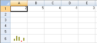
This example creates a column sparkline in a cell and shows negative and series colors.
| C# |  Copy Code Copy Code |
|---|---|
FarPoint.Win.Spread.SheetView sv = new FarPoint.Win.Spread.SheetView(); FarPoint.Win.Spread.Chart.SheetCellRange data = new FarPoint.Win.Spread.Chart.SheetCellRange(sv, 0,0,1, 5); FarPoint.Win.Spread.Chart.SheetCellRange data2 = new FarPoint.Win.Spread.Chart.SheetCellRange(sv, 5,0,1,1); FarPoint.Win.Spread.ExcelSparklineSetting ex = new FarPoint.Win.Spread.ExcelSparklineSetting(); ex.ShowMarkers = true; ex.ShowNegative = true; ex.NegativeColor = Color.Red; // Use with a Column or Winloss type ex.SeriesColor = Color.Olive; fpSpread1.Sheets[0] = sv; sv.Cells[0, 0].Value = 2; sv.Cells[0, 1].Value = 5; sv.Cells[0, 2].Value = 4; sv.Cells[0, 3].Value = -1; sv.Cells[0, 4].Value = 3; fpSpread1.Sheets[0].AddSparkline(data, data2, FarPoint.Win.Spread.SparklineType.Column, ex); |
|
| VB | Copy Code |
|---|---|
Dim sv As New FarPoint.Win.Spread.SheetView() Dim data As New FarPoint.Win.Spread.Chart.SheetCellRange(sv, 0, 0, 1, 5) Dim data2 As New FarPoint.Win.Spread.Chart.SheetCellRange(sv, 5, 0, 1, 1) Dim ex As New FarPoint.Win.Spread.ExcelSparklineSetting() ex.ShowMarkers = True ex.ShowNegative = True ex.NegativeColor = Color.Red ' Use with a Column or Winloss type ex.SeriesColor = Color.Olive FpSpread1.Sheets(0) = sv sv.Cells(0, 0).Value = 2 sv.Cells(0, 1).Value = 5 sv.Cells(0, 2).Value = 4 sv.Cells(0, 3).Value = -1 sv.Cells(0, 4).Value = 3 FpSpread1.Sheets(0).AddSparkline(data, data2, FarPoint.Win.Spread.SparklineType.Column, ex) |
|
Using the Spread Designer
- Type data in a cell or a column or row of cells in the designer.
- Select a cell for the sparkline.
- Select the Insert menu.
- Select a sparkline type.
- Set the Data Range in the Edit Sparklines dialog (such as =Sheet1!$E$1:$E$3).
- Select OK.
- Select Apply and Exit from the File menu to save your changes and close the designer.